Universidade Federal de Santa Maria

Ci. e Nat., Santa Maria v.42, Special Edition: 40 anos, e2, 2020

DOI:10.5902/2179460X39940

ISSN 2179-460X

Received 10/09/19   Accepted: 19/09/20  Published: 03/09/20

 

 

40 years - anniversary

 

The long-term inverse Nakagami distribution: Properties, inference and application

 

A distribuição Nakagami inversa de longo termo: propriedades, inferência e aplicação

 

Francisco Louzada Neto
Pedro Luiz Ramos

Paulo Henrique Ferreira da Silva

 

^I Institute of Mathematical and Computer Sciences, University of São Paulo, São Carlos, Brazil. E-mail: louzada@icmc.usp.br.

^II Institute of Mathematical and Computer Sciences, University of São Paulo, São Carlos, Brazil. E-mail: pedrolramos@usp.br.

^III Institute of Mathematical and Computer Sciences, University of São Paulo, São Carlos, Brazil. E-mail: paulohenri@ufba.br.

 

 

ABSTRACT

In this paper, a new long-term survival distribution, the so-called long-term inverse Nakagami distribution, is presented. The proposed distribution allows us to fit data with unimodal hazard function, where a part of the population is not susceptible to the event of interest, the so-called long-term survival. This distribution can be used, for instance, in clinical studies where a portion of the population can be cured during a treatment. Some mathematical properties of the new distribution are derived. The inferential procedures for the parameters are discussed under the maximum likelihood estimators. A numerical simulation study is carried out to verify the performance of these estimators. Finally, an application to real data on patients’ lifetime after acute myocardial infarction illustrates the usefulness of the proposed distribution.

Keywords: Acute myocardial infarction; Cure fraction; Inverse Nakagami distribution; Long-term survival distribution; Maximum likelihood estimation.

 

RESUMO

Neste artigo, uma nova distribuição de longa duração é introduzida, denominada distribuição de longa duração inversa Nakagami. A distribuição proposta nos permite ajustar dados com a função de risco unimodal, em que uma parte da população não é suscetível ao evento de interesse. Este modelo pode ser usado, por exemplo, em estudos clínicos em que uma parte da população pode ser curada durante um tratamento. Algumas propriedades matemáticas do novo modelo são apresentados. Os procedimentos inferenciais para os parâmetros são discutidos sob os estimadores de máxima verossimilhança. Um estudo de simulação numérica é realizado para verificar o desempenho desses estimadores. Finalmente, uma aplicação a dados reais sobre o tempo de vida de pacientes após infarto agudo do miocárdio ilustra a utilidade do modelo proposto.

Palavras-chave: Infarto agudo do miocárdio; Fração de cura; Distribuição inversa Nakagami; Distribuição de longa duração; Estimação por máxima verossimilhança.

 

 

1 INTRODUCTION

Deriving lifetime distributions has been of great interest among researchers for decades. Lifetime distributions can be motivated by either mathematical or lifetime issues (i.e., physical principles) interest (Ristic´ e Nadarajah, 2014). However, regardless of their motivation, new lifetime distributions are often required in order to provide reasonable fittings for a broad spectrum of real-world datasets. Indeed, real-world datasets may possess peculiar characteristics that can not be appropriately addressed by the existing distributions.

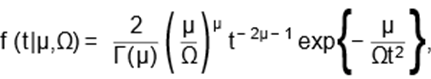
In this sense, Louzada et al. (2018) recently proposed the inverse Nakagami (INK) distribution. Let T be a random variable with an INK distribution, then its probability density function (PDF) is given by

(1)

for all t > 0, where Γ(µ) = e^−tt^µ−1dt is the gamma function, µ > 0 and Ω > 0 are the shape and scale parameters, respectively. The INK distribution contains some important sub-models, such as the inverse Rayleigh (µ = 1), inverse half-normal (µ = 0.5), inverse chi (Ω = 1, µ = ν/2, and ν = 1,2, . . .) and inverse Hoyt (0 < µ < 1) distributions. The authors showed that the INK distribution has unimodal hazard rate function, regardless of the parameter values.

The use of unimodal hazard rate function is very realistic when describing the lifetime of a patient susceptible to disease. For instance, Chowell e Nishiura (2014) argued that Ebola virus has a mean incubation period of 12.7 days, with an infectious mean period of 6.5 days. Additionally, the mean lifetime from illness onset to death is ten days. In this case, the risk of the patient dying from this particular virus first increases over time, but after a period decreases, i.e., it has a unimodal hazard rate. Although Ebola is highly fatal (its fatality ratio is between 61% and 89% in Zaire; see Chowell e Nishiura (2014) and the references therein), the population may not experience the death related to the disease. This characteristic is known as cure fraction.

The long-term survival models, also known as cure rate models, have been widely used in the literature. Berkson e Gage (1952) proposed the existence of two subpopulations, susceptible and non-susceptible to the event of interest, which leads to the standard mixture long-term survival model. Chen et al. (1999) further proposed the promotion time long-term survival model, which is based on the Poisson distribution. Rodrigues et al. (2009) unified the different long-term survival models by using a general structure for the different latent activation mechanisms, which leads to the long-term survival models. Many distributions have been considered as baseline distributions of the models cited above. For instance, Cordeiro et al. (2016) considered the negative binomial distribution for the latent variable distribution, where the baseline survival distribution is the Birnbaum-Saunders. Gallardo et al. (2017) proposed the Pareto IV power series long-term survival model. Ramos et al. (2017) considered the standard mixture long-term survival distribution with the Fréchet distribution, and named it as the long-term Fréchet distribution. Furthermore, the so-called “defective” models have also been used by many authors to describe data with long-term survivals (Balka et al., 2011; Santos et al., 2017; Rocha et al., 2017).

In this paper, we propose the long-term inverse Nakagami (LINK) distribution, which is based on the standard mixture long-term survival distribution, where the baseline distribution is the INK distribution. The INK distribution is useful to describe patients’ lifetime data, where the susceptible group has a unimodal hazard rate. Several mathematical properties of the proposed distribution are derived and discussed. The parameter estimation is considered under the maximum likelihood estimators (MLEs). The LINK distribution is then used to describe the lifetime of patients after acute myocardial infarction in Rio de Janeiro city, Brazil. This dataset was firstly presented in Melo et al. (2004) and indicated an elevated long-term survivals fraction among the patients, which can be accurately estimated by our new distribution.

The remainder of the paper is organized as follows. Section 2 reviews the INK distribution. Section 3 presents the new LINK distribution. Section 4 discusses parameter estimation using the maximum likelihood method. Section 5 introduces a simulation study aiming to verify the performance of the MLEs. Section 6 illustrates the relevance of our proposed methodology in a real lifetime data. Finally, Section 7 summarizes the study.

 

 

2 INK Distribution

The mean and variance of the INK distribution (1) are given, respectively, by

 

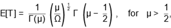
and

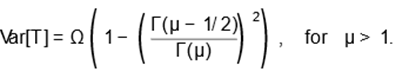
Moreover, its survival and hazard rate functions are given, respectively, by

(2)

and

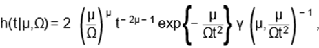
(3)

where γ(y,x) =  w^y−1e^−wdw is the lower incomplete gamma function. As commented before in Section 1, the hazard rate function (3) is unimodal for all µ > 0 and Ω > 0.

The results above, as well as other mathematical properties of the INK distribution, including its r-th moment, r-th central moment, mean residual life function and Shannon’s entropy, are presented in Louzada et al. (2018).

 

 

3 Long-term survival Model

An important characteristic to be taken into account when modeling lifetime data is the existence of long-term survivors, i.e.,   a portion of the population which may not be susceptible to the event of interest (see, e.g., Maller e Zhou, 1995; Perdoná e Louzada-Neto, 2011). In this case, we suppose that the population is split into two groups: those patients that are not susceptible to the event of interest with probability π, and those who are susceptible (in risk) to the event with probability (1 –π). The long-term survival function is then given by

Spop(t) = π + (1 − π)S0(t),

(4)

where π  (0,1) and S₀(t) denotes the baseline survival function for the susceptible group in the population.

The obtained (unconditional) survival function (4), which represents the survival function for the entire population, is improper and lim_t→∞ S_pop(t) = π. From (4), one can easily derive the probability sub-density function (PSDF) given by

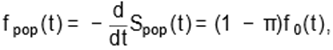
(5)

where f₀(t) is the baseline PDF for the susceptible individuals. Hence, from (4) and (5), we obtain the hazard rate function

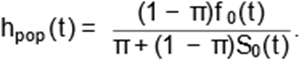
(6)

In this paper, we assume that f₀(t) follows an INK distribution. Then, it follows from (1) and (5) that the PSDF of the LINK distribution is give

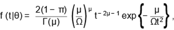
(7)

where θ = (µ, Ω ,π) denotes the parameter vector.

The r-th moment of T is

By considering (2) and (4), we obtain the improper survival function of the LINK distribution

Figure 1 shows the shape of the PSDF and the improper survival function of the LINK distribution, for some parameter values.

 

Figure 1 - Left panel: PSDF of the LINK distribution. Right panel: improper survival function of the LINK distribution. Finally, from (1), (2) and (6), we have the hazard rate function of the LINK distribution

Finally, from (1), (2) and (6), we have the hazard rate function of the LINK distribution:

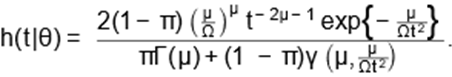
(8)

Note that

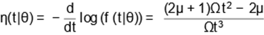
(9)

and

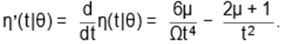
(10)

Glaser (1980) proved that, for a non-negative continuous random variable with twice-differentiable PDF (or PSDF, in our case), if η(t|θ) has a unimodal shape, then h(t|θ) has also a unimodal shape. For all µ > 0 and Ω > 0, we have that (9) is unimodal shaped, with a global maximum at t^∗ =  (which is obtained by equaling (10) to zero). Therefore, (8) is also unimodal shaped. shaped. Figure 2 shows the shape of the hazard function of the LINK distribution.

 

Figure 2 - Hazard shape of the LINK distribution for different values of µ, Ω and π

 

 

4 Inference

Suppose that the lifetime of the i-th patient may not be observed and is subject to right-censoring.  Moreover, consider that the random censoring times C_i’s are independent of the true lifetimes T_i’s, and the distribution of C_i’s does not depend on the parameters governing the distribution of T_i’s.  Then, for a sample of size n, the dataset is  D = {(t_i,δ_i) :  i = 1, . . . ,n} , where   t_i = min {T_i,C_i}  and δ_i = I(T_i≤C_i), with I(.) denoting an indicator function.  This random censoring scheme has as special cases the types I and II censoring schemes. The likelihood function is given by

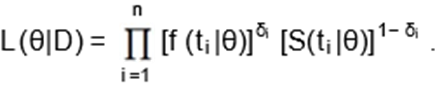
Let T1, . . . ,Tn be a random sample of size n from the LINK distribution (7). Then, the likelihood function, considering data with random censoring, is given by

 

The log-likelihood function is given by

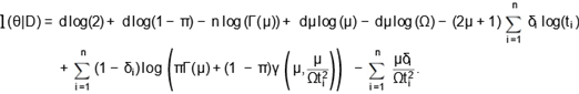
(11)

The maximum likelihood method is the most widely used approach for estimating parameters, since it provides estimators (MLEs) that have several desirable properties, such as asymptotic efficiency, consistency and invariance. The MLEs θˆ of θ are obtained from the solution of ∂l(θ|D)/∂µ = 0, ∂l(θ|D)/∂Ω = 0 and ∂f(θ|D)/∂π  =  0.  Hence, the likelihood equations are given as follows:

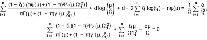
and

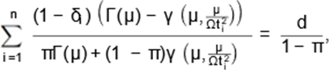
Where  is the digamma function;  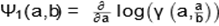and 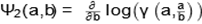 can be calculated numerically. Numerical methods need to be used to find the solution (maximum likelihood estimates) of these nonlinear equations.

Under mild regularity conditions, the MLEs are consistent, efficient and asymptotically normally distributed with a joint trivariate normal distribution given by

θˆ ∼ N₃  θ,I⁻¹(θ) for    n → ∞,

where I(θ) is the 3 × 3 Fisher information matrix for θ, and I_ij(θ) is the (i,j)-th element of I(θ) given by

 

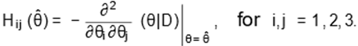
Note, however, that it is not possible to compute the Fisher information matrix I(θ) due to the presence of censored observations (censoring is random and non-informative). Thus, one alternative approach is to use the observed information matrix H(θ) evaluated at θˆ, i.e. H(θˆ), whose terms are given by

Large-sample (approximate) confidence intervals at level 100(1 − ξ)%, for each parameter θ_i, i = 1, 2, 3, can be calculated as

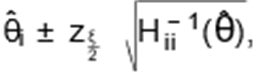
where z_ξ/2 denotes the (ξ/2)-th quantile of a standard normal distribution.

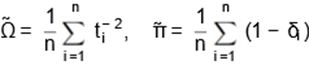
As discussed earlier, we have considered maximization procedures to find the solution of the MLEs. The use of good initial values play an important role to achieve convergence of the estimates with less computational cost. The starting values for Ω and π can be obtained by

(12)

and µ can be estimated by

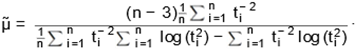
(13)

The initial values for µ and Ω are derived following the closed-form estimators for complete data proposed by Louzada et al. (2018). The initial value for π is obtained as the proportion of censored data (in this case, it is expected that the long-term survivals fraction will be smaller than the proportion of censoring). Observe that we expect to get biased estimates from the equations above. On the other hand, these biased estimates allow us to initiate the Newton-Raphson algorithm closer to the maximum likelihood estimates than using random values.

 

Figure 3 - MREs, MSEs and CPs related to the ML estimates of µ = 0.5, Ω = 2 and π = 0.4, for N = 100,000 simulated samples and different values of n

 

5 Simulation Study

In this section, a Monte Carlo simulation study is provided to investigate the performance of the maximum likelihood (ML) method. This procedure is conducted by computing the mean relative estimate (MRE) and the mean square error (MSE), which are given by

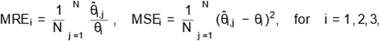
where N = 100,000 is the number of ML estimates (or Monte Carlo samples). Additionally, we compute the coverage probabilities (CPs) of the 95% asymptotic confidence intervals. Under the proposed metrics, we expect that the MLEs return MREs close to one with small MSEs. Moreover, for a 95% confidence level, the proportion of intervals that cover the true parameter value should be close to 0.95.

The parameter values used to perform the simulations are: µ=0.5, Ω =2 and π=0.4 (Figure 3); µ  =  1.5, Ω  =  6 and π = 0.5 (Figure 4); µ=2, Ω=4 and π=0.6 (Figure 5), where n={50,60, . . . ,400} . Note that we have considered the scenarios where the long-term survivals fraction is 0.4, 0.5, and 0.6, respectively. The assumed censoring scheme is random. Hence we may observe different proportions of censoring for each dataset.  In these scenarios, the observed mean proportion  of censorship is roughly 0.454, 0.638, and 0.724, respectively.  It is important to point out that other parameter values were  also considered and similar results were obtained. The R software (R Core Team, 2014) was used to obtain the results, where the maxLik package (Henningsen e Toomet, 2011) was considered to find the maximization of the log-likelihood function (11). Moreover, this procedure is well-behaved, and we have not faced numerical problems, such as failure of convergence or end on multiple maxima.

 

Figure 4 - MREs, MSEs and CPs related to the ML estimates of µ = 1.5, Ω = 6 and π = 0.5, for N = 100,000 simulated samples and different values of n

 

Figures 3 - 5 present the MREs, MSEs and CPs of the ML estimates of µ, Ω and π, for different values of n. The horizontal line in these plots corresponds to MRE, MSE, and CP equal to one, zero and 0.95, respectively. As one can see from these figures, the MLEs of µ, Ω and π are asymptotically unbiased, since the MREs tend to one and the MSEs decrease to zero as n increases. Moreover, with CPs tending to 0.95 when n becomes large, good coverage properties may be deliberated for the MLEs. Thus, in practical applications, the ML estimation method will be relevant, as shown in the next section.

 

Figure 5 - MREs, MSEs and CPs related to the ML estimates of µ = 2, Ω = 4 and π = 0.6, for N = 100,000 simulated samples and different values of n

 

 

6 Acute Myocardial Infarction Data

In this section, we consider a real dataset related to the lifetime (in days) of 3,077 patients after acute myocardial infarction (AMI). They were admitted to the Brazilian National Health System (Sistema Único de Saúde, or SUS in Portuguese), in Rio de Janeiro city, Brazil, during the year 2000. This dataset was firstly analyzed by Melo et al. (2004) and can be fully accessed at http://sobrevida.fiocruz.br/infarto.html.

In order to compare different models (including our proposed LINK distribution), we consider three long-term lifetime distributions: the long-term Fréchet (LF) distribution (Ramos et al., 2017), the well-known long-term Weibull distribution (LW) and the long-term weighted Lindley (LWL) distribution (Louzada e Ramos, 2017). The LF distribution has PSDF given by

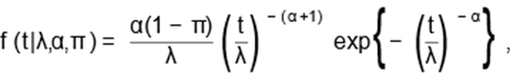
for t > 0, where λ > 0, α > 0 and π ∈ (0,1) are, respectively, the scale, shape and mixing parameters. This distributionparameter estimation under the ML approach is performed using the results presented in Ramos et al. (2017). Additionally, the LW distribution has PSDF given by

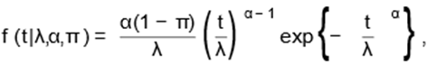
for t,λ,α > 0 and π ∈ (0,1). Finally, the PSDF of the LWL distribution is given by

for t,η,c > 0 and π ∈ (0,1). The inference for this distribution parameters is conducted using the same steps as discussed by the main authors.

The results obtained using the LINK distribution are compared to the corresponding ones achieved with the use of the long-term lifetime models described above. In order to select which distribution to use, we consider different discrimination criteria, such as the AIC (Akaike Information Criterion) and AICc (Corrected Akaike Information Criterion), which are calculated by 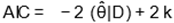 and, where k is the number of parameters to be estimated.  For a set of candidate models that fitted the data at hand, the preferred distribution is the one that provides the minimum AIC and AICc values.

Figure 6 shows the fitted survival functions superimposed to the empirical survival function (Kaplan-Meier estimate). From this figure, we can see that the LINK distribution gives a better fit to the patient’s lifetime data.

Figure 6 - Long-term (improper) survival function adjusted by different distributions and the Kaplan-Meier (KM) estimator,  considering the dataset related to patients’ lifetime after AMI in Rio de Janeiro, Brazil (year 2000)

 

Table 1 presents the negative log-likelihood (-log L), AIC and AICc values for different long-term lifetime models. It can be observed from this table that the LINK distribution provides a better fit to these data since the adjusted distribution has the lowest values in all criteria.

 

Table 1 - The -log L, AIC and AICc values for the fitted distributions, considering the dataset related to patients’ lifetime after AMI in Rio de Janeiro, Brazil (the year 2000)

	LF	LW	LWL	LINK
-log L	2873.4	2933.4	2985.5	2857.4
AIC	5752.8	5872.7	5976.9	5720.9
AICc	5752.8	5872.7	5976.9	5720.9

The parameter estimates of the LINK distribution were obtained using the same procedure as described in Section 4. The initial values determined from (12) and (13) were Ω˜  = 0.03879, π˜  = 0.84433 and µ˜  = 0.14296, and only 10 iterations were necessary to achieve the ML estimates using the Newton-Raphson maximization algorithm. Table 2 exhibits the ML estimates, the standard errors (SE) and the 95% confidence intervals (95% CI) for µ, Ω and π.

 

Table 2 - ML estimates, SE and 95% CI for the parameters of the LINK distribution, considering the proposed dataset

Parameter	Estimate	SE	95% CI
µ	0.1450	0.00061	(0.0966; 0.1935)
Ω	0.1680	0.00051	(0.1238; 0.2123)
π	0.7709	0.00049	(0.7275; 0.8144)

 

The hazard function for the proposed dataset is available in Figure 7. The curve shown in this figure describes the instantaneous death rate for the patients that had AMI. In this case, we can observe that the patients have a higher chance of death in the first days. On the other hand, as time goes by, the hazard rate decreases until they are not susceptible to death by AMI.

 

Figure 7 - Hazard curve of the LINK distribution fitted to the proposed dataset

 

Therefore, through our proposed methodology, the dataset related to the lifetime of patients after AMI in Rio de Janeiro, Brazil, can be well-described by the LINK distribution.

 

 

7 Discussion

In this paper, we have derived a new distribution named long-term inverse Nakagami distribution, which can accommodate long-term survivals fraction in survival analysis. The proposed distribution has unimodal hazard function,  which is realistic  for describing the lifetime of patients that may not experience the event of interest. The mathematical properties of the new distribution were discussed. The maximum likelihood estimators of the parameters and their asymptotic properties were presented. The simulation study showed that the maximum likelihood method provides efficient estimators for unknown parameters and returns good coverage probabilities as the sample size increases.

The long-term inverse Nakagami distribution was used to describe the lifetime of patients that had acute myocardial infarction. In this case, we concluded that the long-term survivals fraction of the patients was 0.7709, i.e., the patients that had not died from that condition.

Many extensions of the present work can be considered. For instance, covariates can be included in the long-term survival term to improve the prediction, e.g., using the logistic link function given by

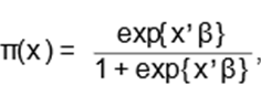
where β = (β₀,β₁, . . . ,β_p) is the vector of parameters related to the vector of covariates x = (1,x₁, . . . ,x_p) . Another approach that can be considered is the use of Bayesian methods to improve the estimates for small samples. Future work will investigate such proposals.

 

 

Disclosure statement

No potential conflict of interest was reported by the authors.

 

 

Acknowledgements

Francisco Louzada and Pedro L. Ramos acknowledge support from the São Paulo State Research Foundation (FAPESP Processes 2013/07375-0 and 2017/25971-0, respectively).

 

 

References

Balka, J., Desmond, A. F., McNicholas, P. D. (2011). Bayesian and likelihood inference for cure rates based on defective inverse Gaussian regression models. Journal of Applied Statistics, 38(1), 127–144.

Berkson, J., Gage, R. P. (1952). Survival curve for cancer patients following treatment. Journal of the American Statistical Association, 47(259), 501–515.

Chen, M. H., Ibrahim, J. G., Sinha, D. (1999). A new Bayesian model for survival data with a surviving fraction. Journal of the American Statistical Association, 94(447), 909–919.

Chowell, G., Nishiura, H. (2014). Transmission dynamics and control of Ebola virus disease (EVD): a review. BMC Medicine, 12(1), 196.

Cordeiro, G. M., Cancho, V. G., Ortega, E. M. M., Barriga, G. D. C. (2016). A model with long-term survivors: negative binomial Birnbaum-Saunders. Communications in Statistics-Theory and Methods, 45(5), 1370–1387.

Gallardo, D. I., Gómez, Y. M., Arnold, B. C., Gómez, H. W. (2017). The Pareto IV power series cure rate model with applications.

SORT-Statistics and Operations Research Transactions, 41(2), 297–318.

Glaser, R. E. (1980). Bathtub and related failure rate characterizations. Journal of the American Statistical Association, 75(371), 667–672.

Henningsen, A., Toomet, O. (2011). maxLik: A package for maximum likelihood estimation in R. Computational Statistics, 26(3), 443–458.

Louzada, F., Ramos, P. L. (2017). A new long-term survival distribution. Biostatistics and Biometrics Open Access Journal, 1(4), 1–6.

Louzada, F., Ramos, P. L., Nascimento, D. (2018). The inverse Nakagami-m distribution: A novel approach in reliability. IEEE Transactions on Reliability, 67(3), 1030–1042.

Maller, R. A., Zhou, S. (1995). Testing for the presence of immune or cured individuals in censored survival data. Biometrics, 51(4), 1197–1205.

Melo, E. C. P., Travassos, C. M. R., Carvalho, M. S. (2004). Infarto agudo do miocárdio no Município do Rio de Janeiro: qualidade dos dados, sobrevida e distribuição espacial. Tese de Doutorado.

Perdoná, G. C., Louzada-Neto, F. (2011). A general hazard model for lifetime data in the presence of cure rate. Journal of Applied Statistics, 38(7), 1395–1405.

R Core Team (2014). R: A Language and Environment for Statistical Computing. (Version 3.3.1). R Foundation for Statistical Computing, Vienna, Austria.

Ramos, P. L., Nascimento, D., Louzada, F. (2017). The long term Fréchet distribution: Estimation, properties and its application.

Biometrics & Biostatistics International Journal, 6(3), 00,170.

Ristic´, M. M., Nadarajah, S. (2014). A new lifetime distribution. Journal of Statistical Computation and Simulation, 84(1), 135–150.

Rocha, R., Nadarajah, S., Tomazella, V., Louzada, F. (2017). A new class of defective models based on the Marshall-Olkin family of distributions for cure rate modeling. Computational Statistics & Data Analysis, 107, 48–63.

Rodrigues, J., Cancho, V. G., de Castro, M., Louzada-Neto, F. (2009). On the unification of long-term survival models. Statistics & Probability Letters, 79(6), 753–759.

Santos, M. R., Achcar, J. A., Martinez, E. Z. (2017). Bayesian and maximum likelihood inference for the defective Gompertz cure rate model with covariates: an application to the cervical carcinoma study. Ciência e Natura, 39(2), 244–258.