Universidade Federal de
Santa Maria
Ci.
e Nat., Santa Maria v.42, Special Edition: 40 anos, e10, 2020
DOI:10.5902/2179460X40100

40 years - anniversary
Four
generalized Weibull distributions: Similar properties and applications
Edwin
Ortega I
Fábio Prataviera
II
Gauss Moutinho
Cordeiro III
I
Universidade
de São Paulo, Piracicaba, Brazil. E-mail: edwin@usp.br.
II
Universidade
de São Paulo, Piracicaba, Brazil. E-mail: fabio_prataviera@usp.br.
III
Universidade
Federal de Pernambuco, Recife, Brazil. E-mail: gauss@de.ufpe.br.
ABSTRACT
We derive a common linear
representation for the densities of four generalizations of the two-parameter
Weibull distribution in terms of Weibull densities. The four generalized
Weibull distributions briefly studied are: the Marshall-Olkin-Weibull,
beta-Weibull, gamma-Weibull and Kumaraswamy-Weibull distributions. We demonstrate
that several mathematical properties of these generalizations can be obtained
simultaneously from those of the Weibull properties. We present two
applications to real data sets by comparing these generalized distributions. It
is hoped that this paper encourage developments of further generalizations of
the Weibull based on the same linear representation.
Keywords: Beta Weibull;
Gamma-Weibull; Kumaraswamy-Weibull; Marshall-Olkin-Weibull.
1 INTRODUCTION
The two-parameter Weibull distribution is named
after Waloddi Weibull pioneered this distribution to model data sets of widely
differing characteristics. Over the last three decades many Weibullrelated
distributions have been constructed with a view for applications in various
areas such as medicine, reliability, engineering, survival analysis,
demography, actuarial study and several others. The Weibull distribution has
been so far the most important distribution for modeling lifetime data and
phenomenon with monotone hazard rates. When modeling these types of hazard
rates, it may be an initial choice because of its negatively and positively
skewed density shapes. Its major weakness is its inability to accommodate
non-monotone hazard rates (in particular, bathtub shaped hazard rates) which
has lead to seek for some of its generalizations.
The first generalization allowing for
non-monotone hazard rates, including the bathtub shaped hazard rate, is the exponentiated
Weibull (EW) distribution pioneered by Mudholkar and Srivastava (1993)
which provides significantly better fits than traditional models based on the
exponential, gamma, Weibull, log-logistic and log-normal distributions.
The cumulative distribution function (cdf) and
probability density function (pdf) of the twoparameter Weibull distribution
(for x > 0) are
|
Gλ,c(x) = 1 − exp[−(λx)c]
|
(1)
|
and
|
gλ,c(x) = cλc xc−1 exp[−(λx)c],
|
(2)
|
respectively, where c > 0 is a shape
parameter and λ > 0 is a scale parameter. Henceforth, we write T ∼
W(λ,c) for a random variable T having density (2). The quantile
function (qf) of T is Qλ,c(u)
= G−λ,c1(u) = λ−1 [−log(1 − u)]1/c.
The paper is unfolded as follows. In Section 2,
we review four generalized Weibull distributions which have been investigated
in the last twenty years based of the families introduced by Marshall and Olkin
(1997), Eugene et al. (2002), Zografos and Balakrishnan (2009) and
Cordeiro and de Castro (2011). We also give simple forms to generate data from
these generalized models. In Section 3, we provide a common linear
representation for the densities of the four generalized distributions in terms
of Weibull densities. Some mathematical properties for all of them can be
determined from this useful linear representation and those Weibull properties
as shown in Section 4. Other extended Weibull distributions are addressed
telegraphically in Section 5. Maximum likelihood estimation is summarized in
Section 6. In Section 7, we compare the four generalized Weibull models by
means of two real life data sets. Finally, Section 8 offers some concluding
remarks.
2 Four generalized Weibull distributions
Henceforth, we consider the Weibull
distribution as defined by (1) and (2) to present four generalized Weibull
distributions.
The first generalization follows the Marshall
and Olkin’s (1997) method to expand a distribution by adding an extra shape
parameter. There are more than 30 published papers on distributions generated
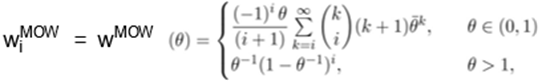
using this method. The cdf of the Marshall-Olkin-Weibull (MOW) distribution
(for θ > 0) can be expressed as
|

|
(3)
|
The quantile function (qf) of the MOW
distribution is easily determined as QMOW(u) = Qλ,c
(θu/[1 − (1 − θ)u]). The density function
corresponding to (3) takes the form
|

|
(4)
|
For θ = 1, fMOW(x)
is equal to gλ,c(x) and, for different values of θ,
fMOW(x) can be more flexible than gλ,c(x).
The hazard rate function (hrf) of the MOW
distribution reduces to
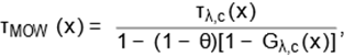
where τλ,c(x) is the
Weibull hrf corresponding to (2).
The last equation implies that τMOW(x)/τλ,c(x)
is increasing in x for θ > 1 and decreasing in x for 0 <
θ < 1. So, the extra parameter θ is called “tilt parameter”,
since the hrf of the MOW distribution is shifted below (θ > 1) or
above (0 < θ < 1) of the Weibull hrf. In fact, for all x > 0,
τMOW(x) ≤ τλ,c(x) when θ ≥
1, and τMOW(x) ≥ τλ,c(x) when
0 < θ ≤ 1. Further details were addressed by Marshall and Olkin
(1997).
The second generalization is the beta-Weibull
(BW) distribution (with four positive parameters) which follows from the
family pioneered by Eugene et al. (2002) by taking the Weibull as the
baseline model. The BW cdf with two additional shape parameters a > 0
and b > 0 is
|
 , ,
|
(5)
|
where B(a,b) = Γ(a + b)/[Γ(a)Γ(b)]
is the beta function, Γ(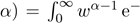 wdw is the gamma function and
 is the
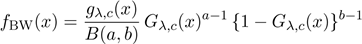
incomplete beta function ratio. The pdf corresponding to (5) has the form
is the
incomplete beta function ratio. The pdf corresponding to (5) has the form
|
 . .
|
(6)
|
The BW distribution includes as special cases
the EW (b = 1), exponentiated exponential (EE) (b = c =
1), Weibull (a = b = 1), exponential (a = b = c =
1), Burr Type X and Type 2 extreme value distributions as well as the
distribution of the order statistic from a Weibull population. Its applications
have been widespread in oncology, finance, system failures, reliability
prediction, extreme value data using floods, models for carbon fibrous
composites, modeling tree diameters, among several others.
The pdf and the hrf of the BW distribution are
obtained from (1), (2), (5) and (6) using Ix(a,b) = I1−x(b,a) as
 ,
,
and
 ,
,
respectively.
The shape of τBW(x) is
constant when a = c = 1, decreasing when ac ≤ 1 and c ≤
1, increasing when ac ≥ 1 and c ≥ 1, bathtub when ac < 1
and c > 1, and unimodal when ac > 1 and c < 1.
The qf of the BW distribution follows easily
from the beta qf. By inverting (5), we can write
 ,
,
where Iu−[1](a,b) denotes the inverse of the incomplete beta function
ratio. Some expansions for
Iu−1(a,b) can be found in Wolfram website1. So, we can
generate BW random variables by
X = λ−1 {−log(1 − V )}1/c ,
where V is a beta variate with shape
parameters a and b.
The third
generalization follows from Zografos and Balakrishnan’s (2009) gamma family
with an extra shape parameter a > 0. The cdf of the gamma-Weibull
(GW) distribution is
|

|
(7)
|
where tdt is the lower incomplete gamma
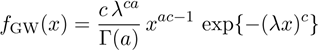
function. The GW density takes the
tdt is the lower incomplete gamma
function. The GW density takes the
form
|
 . .
|
(8)
|
A physical motivation for the GW distribution
can follow from Zografos and Balakrishnan (2009): if XL(1),...,XL(n)
are lower record values from a sequence of independent random variables
with common Weibull pdf gλ,c(x), then the pdf of the nth
lower record value has the form (8). If Z is a gamma random variable
with unit scale parameter and shape parameter a > 0, then X = Qλ,c(eZ)
has density (8). So, the GW distribution is easily generated from the gamma
distribution and the Weibull qf.
Further, the GW density function (for x >
0) can be expressed as
|
|
(9)
|
Equation (9) extends some distributions
previously discussed in the literature. In fact, it is identical to the
generalized gamma distribution (Stacy, 1962). The Weibull distribution is a
basic exemplar when a = 1, whereas the gamma distribution follows when c
= 1. The half-normal distribution is obtained for a = 3 and c =
2. In addition, the log-normal distribution is a limiting special case when a
tends to infinity.
By inverting (7), the qf of the GW distribution
follows as
|

|
(10)
|
for 0 < u < 1, where Q−1(a,u) is the inverse function
of Q(a,x) = 1 γ(a,x)/Γ(a), see
http:// functions.wolfram.com/ GammaBetaErf/ InverseGammaRegularized/ for
details. Further, the simulation of the GW random variable is quite easy: if V
is a gamma random variable with shape parameter a and unit scale
parameter, then X = λ−1 V 1/c will have the density (9).
Finally, the fourth generalization is the Kumaraswamy-Weibull
(KwW) distribution (with four positive parameters) defined from Cordeiro
and de Castro’s (2011) family by the cdf and pdf
|

|
(11)
|
and
|

|
(12)
|
respectively. Then, the KwW density (for x
> 0) follows from (1), (2) and (12) as
 .
.
It contains as special cases the EW (b =
1), Kumaraswamy exponential (c = 1), exponentiated Rayleigh,
exponentiated exponential, Weibull, Rayleigh and exponential distributions. It
allows for bathtub shaped, monotonically decreasing, monotonically increasing,
and upside down bathtub shaped hazard rates.
The role of the two extra parameters a and
b is to govern skewness and obtain the KwW distributions with heavier or
ligther tails than the Weibull distribution. In fact, the tails of fKwW(x)
will be lighter than those of gλ,c(x) if a > 1
or b > 1. On the other hand, the tails of fKwW(x)
will be heavier than those of gλ,c(x) if a < 1
or b < 1.
The qf of the KwW distribution is readily
obtained from the Weibull qf. In fact, the qf corresponding to (11) is

Further, we can generate
KwW variates by
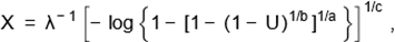
where U is a uniform variate on the unit
interval (0,1).
3 Linear Representations
The four generalized Weibull densities defined
previously can be written as a common linear combination of Weibull densities
whose coefficients depend only on the parameters of the generator family.
The cdf and pdf of the EW distribution with
power parameter α > 0 have the forms
|
Πα,λ,c(x)
= Gλ,c(x)α
|
and
|
πα,λ,c(x) = αGλ,c(x)α−1
gλ,c(x),
|
respectively.
We can expand Πα,λ,c(x)
from (1) using the power series for real non-integer α > 0
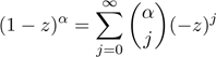
for | z |< 1. Then, we can
write
|

|
(13)
|
where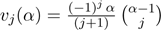 , and gλj,c(x) is the Weibull pdf (1) with scale parameter λj =
(j+1)1/cλ and shape parameter c.
, and gλj,c(x) is the Weibull pdf (1) with scale parameter λj =
(j+1)1/cλ and shape parameter c.
The following four linear representations for
the generalized Weibull distributions described in Section 2 are derived by
using the linear combinations of the family densities provided by some authors
in conjunction with Equation (13). These linear representations for the four
densities in terms of Weibull densities are important to determine their
mathematical properties from those of the Weibull distribution.
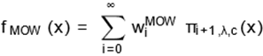
First, based upon the general expansion by
Cordeiro et al. (2014), the MOW density (4) can be expressed as
where the coefficients are (for i= 0,
1, …)
and θ¯ = 1 −
θ. By inserting (13) in the last expression for fMOW(x)
and changing the sums 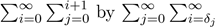 , where δj = 0 for j =
0,1 and δj = j − 1 for j ≥ 2, we obtain
, where δj = 0 for j =
0,1 and δj = j − 1 for j ≥ 2, we obtain
|
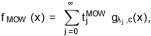
|
(14)
|
where tMOWj 
Second, for the BW density (6), we obtain from
Nadarajah et al. (2012)
|

|
(15)
|
where

By combining (15) and (13), we can easily write
|
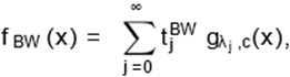
|
(16)
|
where
Third, the linear combination for the GW
density (9) follows from Castellares and Lemonte (2015) as
|
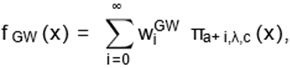
|
(17)
|
where
 ,
,
and ψi−1(·)
are the Stirling polynomials given by
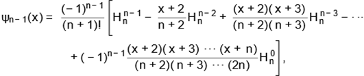
and Hnm are
positive integers given recursevily by  , with
By combining (17) and (13), we obtain (for a
> 0 real non-integer)
|
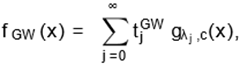
|
(18)
|
where
For the last generalization, the KwW density
(12) can be expressed (Nadarajah et al., 2012) as
|
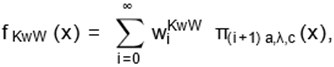
|
(19)
|
where

By combining (19) and (13), we obtain
|
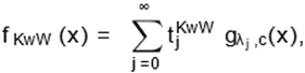
|
(20)
|
where 
Equations (14), (16), (18) and (20) have
identical linear combinations of Weibull densities with
just different coefficients. They can be reduced to a simple equation
|
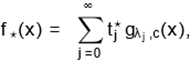
|
(21)
|
where ⋆ stands for any of the four generalized Weibull distributions. So,
whenever possible, several mathematical properties for these generalized
distributions can be determined in a similar manner from those Weibull
properties.
4 Mathematical properties
In this section, we present the main properties
of the Weibull distribution which can be used in the linear representation (21)
to obtain those properties for the MOW, BW, GW and KwW distributions.
Some of the most important features of a
distribution can be studied through moments. The nth ordinary moment of T
∼ W(λ,c) is E(Tn) = λ−n Γ(n/c + 1). Then, the
moments of the four generalized Weibull distributions take the common form
|

|
(22)
|
So, their cumulants (κn) can
be found recursively from , where
 . The skewness
 and
kurtosis
and
kurtosis can be calculated from the third and fourth
standardized cumulants.
can be calculated from the third and fourth
standardized cumulants.
The nth incomplete moment of , is
easily found changing variables from the lower incomplete gamma function as mn(y)
= λ−n γ(n/c
+ 1,(λz)c). Then, the incmomplete moments
of the four generalized Weibull distributions reduce to
, is
easily found changing variables from the lower incomplete gamma function as mn(y)
= λ−n γ(n/c
+ 1,(λz)c). Then, the incmomplete moments
of the four generalized Weibull distributions reduce to
|

|
(23)
|
The first incomplete moment m⋆,1(z) is used to construct the
Bonferroni and Lorenz curves (popular measures in economics, reliability,
demography, insurance and medicine) and to determine the totality of deviations
from the mean and median of a distribution.
For a given probability π, the
Bonferroni and Lorenz curves of any of these four generalized
Weibull distributions are given by ) and L⋆(π) = π B⋆(π),
respectively, where q = Q⋆(π)
is the qf of the chosen distribution (Section 2).
) and L⋆(π) = π B⋆(π),
respectively, where q = Q⋆(π)
is the qf of the chosen distribution (Section 2).
The total deviations from the mean and median
for any of these four generalizations can be expressed as ) and
) and ), where
 )
can be determined for the cdf chosen (Section 2).
)
can be determined for the cdf chosen (Section 2).
We provide two expressions for the moment
generating function (mgf) of T, say Mλ,c(t) = E(etT).
We can write
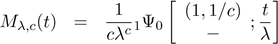
A first representation for Mλ,c(t)
is obtained from the Wright generalized hypergeometric function, namely
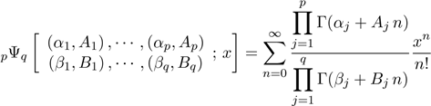 .
.
The Wright function exists if 1 + 0. For c
> 1, we have
0. For c
> 1, we have

and then
 .
.
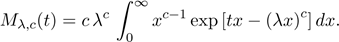
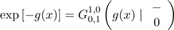
A second representation for M(t)
is based on the Meijer G-function defined by

where i = √−1 is the complex unit and L denotes
an integration path (see Section 9.3 in Gradshteyn and Ryzhik (2000) for a
description of this path). The Meijer G-function contains many integrals with
elementary and special functions (Prudnikov et al., 1986). For an
arbitrary function g(·), based on the result
 ,
,
we can write Mλ,c(t)
as

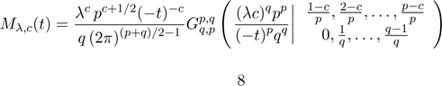
We now assume that c = p/q, where
p ≥ 1 and q ≥ 1 are co-prime integers. Note that this condition
for calculating the integral Mλ,c(t) is not
restrictive since every real number can be approximated by a rational number. Using
equation (2.24.1.1) in Prudnikov et al. (1986, volume 3), we obtain
 .
.
Then, the generating functions of the four
generalized distributions can be written as
 ,
,
where Mλj,c(t) follows from the two expressions for Mλ,c(t)
given before with λ = λj.
5 Other extended Weibull distributions
A first distribution closely related to the EW
distribution is the generalized Weibull distribution pioneered by
Mudholkar et al. (1996) with cdf (for x > 0)

where λ > 0, c > 0 and α
> 0. This distribution allows for bathtub shaped, monotonically
increasing, monotonically decreasing and constant hazard rates.
Gera (1997) presented a modification of the EW
cdf given by F∗(x) = exp(−sxr)Gλ,c(x)α
for r > 0 and s > 0. Lai et al. (2003)
introduced the modified Weibull (MW) density (for x > 0) f(x)
= α(c + δx)xc−1 exp(δx)exp[−αxc exp(δx)], where α
> 0, c > 0 and δ > 0, which allows for increasing
and bathtub shaped hazard rates.
Nadarajah and Kotz (2005) proposed a
four-parameter generalized Weibull-Gompertz distribution with cdf (for x
> 0)

Again, this cdf can lead to increasing,
decreasing or bathtub-shaped hazard rates.
Bebbington et al. (2007) defined the flexible
Weibull density (for x > 0) as

Carrasco et al. (2008) defined the generalized
modified Weibull (GMW) density (for x > 0) as
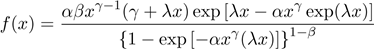 ,
,
where α > 0, γ ≥ 0, λ ≥
0 and β > 0.
Nikulin and Haghighi (2009) proposed the cdf of
the power generalized Weibull distribution (for x > 0) as F(x)
= 1 − exp{1 − [1 + (λx)ν]1/γ}, where
ν > 0, γ ≥ 0 and λ > 0, which allows for increasing,
decreasing, constant, bathtub shaped, and unimodal hazard rates.
Further, Barreto-Souza et al. (2010)
defined the four-parameter beta generalized exponential (BGE) density
(for x > 0) as
 ,
,
where a > 0, b > 0, α
> 0 and λ > 0. The BGE model allows for bathtub shaped,
monotonically increasing, monotonically decreasing and upside-down bathtub
hazard rates.
Silva et al. (2010) introduced the
five-parameter beta modified Weibull (BMW) density (for x > 0)
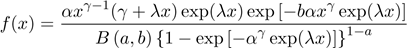
where a > 0, b > 0, α
> 0, γ > 0 and λ ≥ 0. The BMW distribution includes as
sub-models seventeen known distributions such as the EW, BW, MW and GMW
distributions, among others. It allows for bathtub shaped, monotonically
decreasing, monotonically increasing, and upside down bathtub shaped hazard
rates.
Pascoa et al. (2011) defined the
five-parameter Kumaraswamy-generalized gamma density (for x > 0)
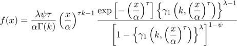 ,
,
where γ1(p,x) = γ(p,x)/Γ(p),
α > 0, λ > 0, k > 0, ψ > 0 and τ
> 0. This distribution contains as special cases the exponentiated
generalized gamma (Cordeiro et al., 2011b) and KwW distributions, among
several others. It allows for constant, bathtub shaped, monotonically
decreasing, monotonically increasing, and upside down bathtub shaped hazard
rates.
Cordeiro et al. (2011c) proposed the beta
extended Weibull family density (for x > 0) by
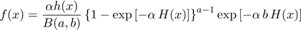 ,
,
where a > 0, b > 0 and α
> 0, H(x) ≥ 0 is a monotonic increasing function of x and
h(x) = dH(x)/dx. This family contains as
sub-models the EW and BMW distributions and also give rise to many new classes
of distributions.
Finally, Alexander et al. (2012) proposed
a class of generalized beta-generated densities given by f∗(x) = cg(x)G(x)ac−1 [1 − G(x)c]b−1/B(a,b)
for shape parameters a > 0, b > 0 and c > 0,
where G(·) is a valid cdf and g(·) is its pdf. Two important
special cases are the beta and Kumaraswamy generated families discussed in
Section 2.
6 Maximum Likelihood Estimation
The parameters of the MOW, BW, GW and KwW
distributions are estimated by maximum likelihood from complete samples only.
Let x1,··· ,xn be a random sample of
size n from the distributions given by (4), (6), (8) and (12) and
parameter vector η. Let q denote the dimension of η.
Parametric inference for such data is usually based on likelihood methods and
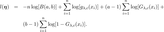
asymptotic theory. The log-likelihoods (l(η)) for the
model parameters are
·For the MOW
distribution, η
= (λ,c,θ)T
 .
.
·For the BW distribution, η = (λ,c,a,b)T
·For the GW
distribution, η
= (λ,c,a)T
 .
.
·For the KwW
distribution, η
= (λ,c,a,b)T
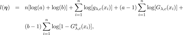
where Gλ,c(xi)
and gλ,c(xi) are defined in Section 1.
The function l(η) can be
maximized either directly by using well-known platforms such as the R (optim
function), SAS (PROC NLMIXED), Ox
program (MaxBFGS sub-routine) or by
solving the nonlinear likelihood equations ∂l(η)/∂η = 0. These equations cannot be solved analytically
numerically. We can use iterative techniques such as the Newton-Raphson type
algorithms withb and statistical software can be used to obtain the maximum
likelihood estimate (MLE) η
of η
initial values for the parameters taken from
the fitted Weibull distribution.
For interval estimation and hypothesis tests on
the model parameters, we require the observed information matrix since its
expectation requires numerical integration. Under standard regularity
conditions that are fulfilled for parameters in the interior of the parameter
space but not on the boundary, the asymptotic distribution of
where I(η) is the
expected information matrix. This asymptotic behavior is valid if I(η) is reNq(0,J(η)−1)b distribution can be used to
construct approximate confidence intervals and confib placed by J(η), i.e., the observed information matrix evaluated at η. The multivariate normal dence regions for the individual
parameters and for the hazard rate and survival functions.
7 Applications
All generalized distributions mentioned
previously can be fitted to real data sets using the AdequacyModel package
by the BFGS method in the R
software.
In this section, we provide two applications
comparing the four generalized distributions (MOW, BW,GW, KwW) by means of two
real data sets. We calculate the MLEs of the parameters for the fitted
distributions, their standard errors (SEs) (in parentheses) and the following
goodness-of-ft measures: the Akaike Information Criterion (AIC), Bayesian
Information Criterion (BIC), Cram´ervon Misses (W*) statistic and Anderson
Darling (A*) statistic using the AdequacyModel package. The better fits
to the data correspond to small values of these measures.
7.1 Application 1: Repair time data
The following maintenance data refer to active repair
times (in hours) for an airborne communication transceiver. The 45 repair times
analyzed by Chhikara and Folks (1977) are: 0.2, 0.3, 0.5, 0.5, 0.5, 0.5, 0.6,
0.6, 0.7, 0.7, 0.7, 0.8, 0.8, 1.0, 1.0, 1.0, 1.1, 1.3, 1.5, 1.5, 1.5, 1.5, 2,
2, 2.2, 2.5, 2.7, 3.0, 3.0, 3.3, 3.3, 4.0, 4.0, 4.5, 4.7, 5.0, 5.4, 5.4, 7.0,
7.5, 8.8, 9.0, 10.3, 22.0, 24.5.
The results from some fitted distributions to
these data are listed in Table 1. We can note that the KwW model is the most
adequate distribution to these data. The four statistics are favorable when
compared to the nested Weibull distribution. For non-nested models, the
statistics W∗ and A∗ are
favorable to the KwW model with the smallest values.
Table 1 - MLEs of the model parameters for the
repair time data, their SEs (given in parentheses) and statistical measures
|
Model
|
c
|
λ
|
a
|
b
|
AIC
|
BIC
|
W∗
|
A∗
|
|
BW
|
0.591
|
8.849
|
7.964
|
0.227
|
207.39
|
214.70
|
0.041
|
0.282
|
|
|
(0.179)
|
(0.051)
|
(2.311)
|
(0.209)
|
|
|
|
|
|
KwW
|
0.597
|
9.999
|
11.830
|
0.200
|
206.86
|
214.17
|
0.037
|
0.256
|
|
|
(0.177)
|
(0.358)
|
(4.667)
|
(0.188)
|
|
|
|
|
|
GW
|
0.457
|
8.022
|
4.041
|
-
|
209.39
|
214.87
|
0.081
|
0.551
|
|
|
(0.060)
|
(7.543)
|
(1.083)
|
(-)
|
|
|
|
|
|
EW
|
0.545
|
1.198
|
3.260
|
-
|
208.78
|
214.26
|
0.075
|
0.509
|
|
|
(0.121)
|
(0.928)
|
(1.760)
|
(-)
|
|
|
|
|
|
Weibull
|
0.898
|
0.294
|
1
|
1
|
212.93
|
216.59
|
0.129
|
0.900
|
|
|
(0.095)
|
(0.051)
|
(-)
|
(-)
|
|
|
|
|
|
Model
|
c
|
λ
|
θ
|
|
AIC
|
BIC
|
W∗
|
A∗
|
|
MOW
|
1.484
|
0.053
|
0.033
|
|
207.71
|
213.19
|
0.069
|
0.438
|
|
|
(0.204)
|
(0.043)
|
(0.051)
|
|
|
|
|
|
The histogram and the plots of the fitted KwW
and Weibull densities are displayed in Figure 1a. The plots of the empirical
survival and estimated survivals are displayed in Figure 1b. The plots of the
empirical hazard and estimated hazards are displayed in Figure 1c. We conclude
from these plots that the KwW distribution is very suitable to these data.
7.2 Application 2: Chlorobenzene data
In this application, the data refer to a sample
with chlorobenzene concentrations in the air of a factory (in TWAs/15min). The
31 observations represent the average concentrations calculated every fifteen
minutes in an eight-hour shift (Kumagai and Matsunaga, 1995). The averages are:
13.7, 10.2, 9.9, 4.3, 5.6, 45.6, 42.0, 14.1, 3.8, 9.3, 10.6, 91.3, 2.2, 3.8,
6.0, 17.8, 131.8, 31.0, 4.2, 2.6, 27.6, 1.7, 7.0, 2.1, 1.5, 7.5, 2.5, 2.4,
51.9, 12.9, 12.3.
Figure 1 - Plots for repair time data. (a)
Estimated KwW and Weibull densities. (b) Estimated survivals of the KwW and
Weibull distributions. (c) Estimated hazards of the KwW and Weibull
distributions
The results from some fitted distributions to
these data are listed in Table 2. We conclude that the KwW model is the most
suitable to these data. The four statistics are favorable when compared to the
nested Weibull distribution. For non-nested models, the measures W∗ and
A∗ are favorable for the KwW
model with the smallest values.
Table 2 - MLEs of the model parameters for the
chlorobenzene data, their SEs (given in parentheses) and statistical measures
|
Model
|
c
|
λ
|
a
|
b
|
AIC
|
BIC
|
W∗
|
A∗
|
|
BW
|
0.558
|
3.217
|
11.843
|
0.181
|
241.23
|
246.96
|
0.039
|
0.291
|
|
|
(0.072)
|
(0.096)
|
(5.373)
|
(0.085)
|
|
|
|
|
|
KwW
|
0.532
|
5.037
|
27.757
|
0.161
|
240.19
|
245.92
|
0.033
|
0.248
|
|
|
(0.026)
|
(0.028)
|
( 0.001)
|
(0.040)
|
|
|
|
|
|
GW
|
0.316
|
38.670
|
6.854
|
-
|
242.76
|
247.06
|
0.078
|
0.539
|
|
|
(0.019)
|
(0.002)
|
(0.793)
|
(-)
|
|
|
|
|
|
EW
|
0.284
|
8.949
|
21.677
|
-
|
240.02
|
244.33
|
0.042
|
0.319
|
|
|
(0.080)
|
(0.493)
|
(3.100)
|
(-)
|
|
|
|
|
|
Weibull
|
0.820
|
0.059
|
1
|
1
|
245.95
|
248.82
|
0.149
|
0.943
|
|
|
(0.106)
|
(0.013)
|
(-)
|
(-)
|
|
|
|
|
|
Model
|
c
|
λ
|
θ
|
|
AIC
|
BIC
|
W∗
|
A∗
|
|
MOW
|
1.416
|
0.008
|
0.025
|
|
241.6
|
245.90
|
0.052
|
0.394
|
|
|
(0.224)
|
(0.006)
|
(0.035)
|
|
|
|
|
|
The histogram and the plots of the fitted KwW and
Weibull densities are displayed in Figure 2a. The plots of the empirical cdf
and estimated cdfs are given in Figure 2b. The plots of the empirical hazard
and estimated hazards are displayed in Figure 2c. We conclude from these plots
that the KwW distribution is very suitable to these data.
Figure 2 - Plots for chlorobenzene data. (a)
Estimated KwW and Weibull densities. (b) Estimated cdfs of the KwW and Weibull
distributions. (c) Estimated hazards of the KwW and Weibull distributions
8 Conclusions
In this paper, we present a simple linear
representation which holds for the densities of various extensions of the
Weibull distribution. It involves coefficients that depend only on the
parameters of the families and the Weibull densities in convenient forms. We
demonstrate the usefulness of this representation for the he
Marshall-Olkin-Weibull, beta-Weibull, gamma-Weibull and Kumaraswamy-Weibull
distributions. However, it can be valid for some other generalized Weibull
distribution. The main advantage of the linear representation is to derive
easily some mathematical properties for these four distributions from those
Weibull properties. We present two applications of these generalized
distributions to real data sets.
References
Alexander,
C., Cordeiro, G. M., Ortega, E. M. M. and Sarabia, J. M. (2012). Generalized beta-generated
distributions. Computational Statistics and Data Analysis, 56,
1880-1897.
Barreto-Souza, W.,
Santos, A. and Cordeiro, G. M. (2010). The beta generalized exponential distribution.
Journal of Statistical Computation and Simulation, 80, 159-172.
Bebbington, M., Lai, C.D.
and Zitikis, R. (2007). A flexible Weibull extension. Reliability
Engineering and System Safety, 92, 719-726.
Carrasco, J. M. F., Ortega, E. M. M.
and Cordeiro, G. M. (2008). A
generalized modified Weibull distribution for lifetime modeling. Computational
Statistics and Data Analysis, 53, 450-462.
Castellares, F. and
Lemonte, A. (2015). A new generalized Weibull distribution generated by gamma
random variables. Journal of the Egyptian Mathematical Society, 23,
382-390.
Chhikara, R. S. and
Folks, J. L. (1977). The Inverse Gaussian Distribution as a Lifetime Model. Technometrics,
19, 461.
Cordeiro, G. M. and de
Castro, M. (2011). A new family of generalized distributions. Journal of
Statistical Computation and Simulation, 81, 883-898.
Cordeiro, G. M., Ortega,
E. M. M. and Silva, G. (2011b). The exponentiated generalized gamma
distribution with application to lifetime data. Journal of Statistical
Computation and Simulation, 81, 827-842.
Cordeiro, G. M., Ortega,
E. M. M. and Silva, G. (2011c). The beta extended Weibull family. Journal of
Probability and Statistical Science, 10, 15-40.
Cordeiro, G. M., Lemonte,
A. and Ortega, E. M. M. (2014). The Marshall–Olkin Family of Distributions:
Mathematical Properties and New Models. Journal of Statistical Theory and
Practice, 8, 343-366.
Cordeiro, G. M., Lemonte,
A. and Ortega, E. M. M. (2014). The Marshall–Olkin family of distributions:
Mathematical properties and new models. Journal of Statistical Theory and
Practice, 8, 343-366.
Eugene, M, Lee, C. and
Famoye, F. (2002). Beta-normal distribution and its applications. Communication
in Statistics - Theory Methods, 31, 497-512.
Gera, A. W. (1997). The
modified exponentiated-Weibull distribution for lifetime modeling. In: 1997
Proceedings of the Annual Reliability and Maintainability Symposium, pp.
149-152.
Kumagai, S. and
Matsunaga, I. (1995). Changes in the distribution of short-term exposure
concentration with different averaging times. American Industrial Hygiene
Association Journal, 56, 24- 31.
Lai, C. D., Xie, M. and
Murthy, D. N. P. (2003). A modified Weibull distribution. IEEE Transactions
on Reliability, 52, 33-37.
Marshall, A. W., Olkin,
I. (1997). A new method for adding a parameter to a family of distributions
with application to the exponential and Weibull families. Biometrika, 84,
641652.
Mudholkar, G. S. and
Srivastava, D. K. (1993). Exponentiated Weibull family for analyzing bathtub
failure-rate data. IEEE Transactions on Reliability, 42, 299-302.
Mudholkar, G. S. and
Hutson, A. D. (1996). The exponentiated Weibull family: some properties and a
flood data application. Communications in Statistics—Theory and Methods,
25, 3059-3083.
Nadarajah S. and Kotz S.
(2005). On some recent modifications of Weibull distribution. IEEE
Transactions on Reliability, 54, 561-562.
Nadarajah, S., Cordeiro,
G. M., and Ortega, E. M. M. (2012). General results for the Kumaraswamy G distribution.
Journal of Statistical Computation and Simulation, 82, 951-979.
Nikulin, M. and Haghighi,
F. (2009). On the power generalized Weibull family. Metron, 67, 75-86.
Pascoa, M. A. P., Ortega, E. M. M.
and Cordeiro, G. M. (2011). The
Kumaraswamygeneralized gamma distribution with application in survival
analysis. Statistical Methodology, 8, 411-433.
Prudnikov, A. P.,
Brychkov, Y. A. and Marichev, O. I. (1986). Integrals and Series, volumes 1,
2 and 3. Gordon and Breach Science Publishers, Amsterdam.
Silva, G. O., Ortega, E. M. M. and
Cordeiro, G. M. (2010). The
beta modified Weibull distribution. Lifetime Data Analysis, 16,
409-430.
Stacy, E. W. (1962). A
generalization of the gamma distribution. Annals of Mathematical Statistics,
33, 1187-1192.
Zografos, K. and
Balakrishnan, N. (2009). On families of beta- and generalized gamma generated
distributions and associated inference. Statistical Methodology, 6, 344-362.